| 일 | 월 | 화 | 수 | 목 | 금 | 토 |
|---|---|---|---|---|---|---|
| 1 | 2 | 3 | 4 | 5 | ||
| 6 | 7 | 8 | 9 | 10 | 11 | 12 |
| 13 | 14 | 15 | 16 | 17 | 18 | 19 |
| 20 | 21 | 22 | 23 | 24 | 25 | 26 |
| 27 | 28 | 29 | 30 |
- 가중 최소제곱법
- weighted least-squares
- 선형 상수계수 미분방정식#lccode#sinusoidal input
- 푸리에 정리
- reflection matrix
- 선형시스템연산자#라이프니츠 법칙#fundamental theorem of algebra#erf
- 오일러-코시 미방#계수내림법
- 추정문제#normal equation#직교방정식#정사영#정사영행렬#정사영 변환
- dirichlet
- 그람-슈미트 과정#gram-schmidt process
- 여인수 행렬
- 미분방정식 #선형 미분방정식 #상미분 방정식
- 내적#duality#쌍대성#dot product
- 2계미방#모드#mod#특성방정식#characteristic eq#제차해
- 내적 공간#적분
- 정규직교행렬
- linespectra#feurierseries#푸리에 급수
- 상태천이행렬#적분인자법#미정계수법#케일리-헤밀톤 정리
- 선형변환#contraction#expansions#shears#projections#reflection
- 선형독립#기저벡터#선형확장#span#basis
- 계수내림법#reduction of order#wronskian#론스키안#아벨항등식#abel's identity
- 여인자
- 변수분리#동차 미분방정식#완전 미분방정식
- 멱급수법
- 직교행렬#정규직교행렬#orthonormal#reflection matrix#dcm
- 최소자승#least-square#목적함수#양한정#정점조건#최소조건
- 비제차#제차해#일반해#적분인자#적분인자법#homogeneous sol#nonhomogeneous sol#integrating factor
- 베르누이 미분방정식
- 푸리에 급수
- 부분 분수분해
OnlyOne
Pole and Time Constant(시상수) 본문
Pole and Time Constant(시상수)
Taesan Kim 2024. 8. 2. 21:02Pole and Time Constant(시상수)
Pole을 이해하기 위해 Real Exponential Signal에 대한 이해가 필수적이다.
2024.08.02 - [제어공학] - [졸빠거]Exponential Signal
[졸빠거]Exponential Signal
[졸빠거]Exponential Signal제어공학에서 Real Exponential Signal은 제어 시스템의 빠르기 비교에 이용하려는 목적이다.-졸빠거 Real Exponential SignalElementary CT Signals에는 step, ramp 신호, rectangular and triangular
taesan5435.tistory.com
Definition
Pole
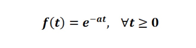
저번 시간에 살펴봤던 Real Exponential Signal의 정의이다. 위 정의에서 Pole은 함수 f의 지수부분에서 t를 제외한 -a이다.
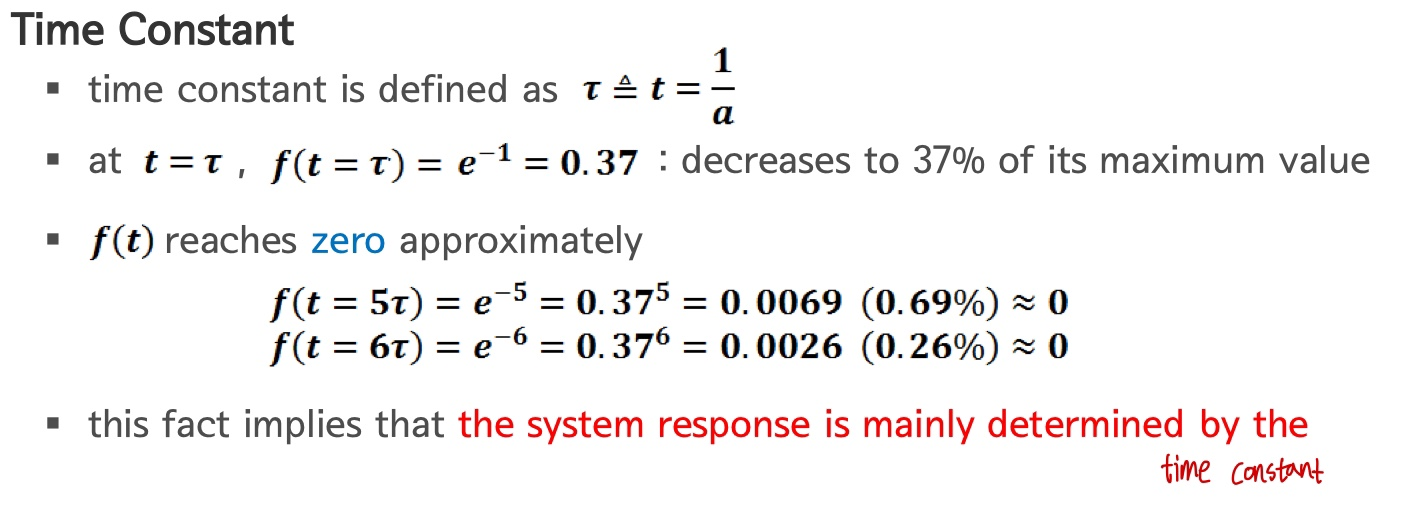
Time Constant(시상수)
1/a와 같다. 흔히 로마자 '타우'로 표현한다.
따라서 Pole이 작아지면, Time Constant(시상수)역시 작아진다.
이게 중요한 이유는 Pole의 비교를 통해 Dominent Pole을 찾고, Stable한 구간에서 Dominent한 신호를 특정할 수 있기 때문이다.
또한 시상수(Time Constant)는 신호가 처음의 37%크기로 줄어드는데 걸리는 시간을 의미하기도 한다. (1/e가 0.37이기 때문이다.)
이것을 다시 정리하면 아래와 같다.
Speed of Signal
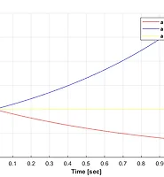
신호의 속도에 관한 비유는 토끼와 거북이에 관한 비유와 같다. 만약 Pole(일반적으로 음수)이 -2이고, -0.1인 두 신호가 있다고 하자.
clc; clear all; close all;

TIME = struct('Start', 0.0, ...
              'Final', 1.0, ...
              'Ntime', 1, ...
              'Ts', 1e-3, ...
              'time', 0);
TIME.time = TIME.Start : TIME.Ts : TIME.Final;
TIME.Ntime = length(TIME.time);

TIME.idx = 1;
t = TIME.time;

a = -0.1;
b = -2;

figure, hold on, grid on;

plot(TIME.time, exp(a*t), 'r-', 'DisplayName', 'pole = -0.1(tortoise)');
plot(TIME.time, exp(b*t), 'b-', 'DisplayName', 'pole = -2(hare)');

%axis equal;

xlabel('Time [sec]', 'FontWeight', 'bold');
ylabel('Amplitude [-]', 'FontWeight', 'bold');
legend('Location', 'northeast', 'FontWeight', 'bold');
토끼와 거북이의 시상수 차이는 20배가 차이난다. 거북이 입장에서는 토끼가 눈에 보이지 않을 것이다. 또한 '일정한 시간'이 지났을 때, 토끼는 거의 보이지 않지만, 여전히 거북이는 보이는 시점이 있다. 이때 거북이를 Dominent하다고 정의하며, 이때의 Pole을 Dominent Pole이라고 한다.
Q. 그렇다면 토끼와 거북이가 모두 보이지 않는 시간(신호의 크기가 무시할 수 있는만큼 줄어드는 시간)은 언제일까?
: 이 시간은 Dominent Pole의 Time Constant를 5~6배한 값이다.
직관적인 이해를 위해 예시를 들어보자.
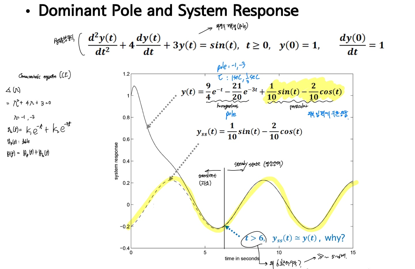
위 상미분방정식을 풀면, Particular Solution(특성해)과 Homogenious Solution(동차해)의 합으로 이루어진 General Solution(일반해)이 나온다. 여기서 Homogenious Solution은 시간이 지나면 Pole에 의해 정상상태로 수렴한다.
이때, 언제부터를 정상상태로 볼 것이냐? 하는 질문이 생기는데, 이것의 기준이 되는 값이 Dominent Pole이다.
위 예시에서는 시상수가 1초이고, 시상수의 6배인 6초부터 Steady State인 것을 확인할 수 있다.
이를 실제로 Matlab시뮬레이션을 돌렸다.
2024.08.16 - [Engineering/Matlab Simulation] - Dominant Pole Concept
Dominant Pole Concept
Dominant Pole Concept2024.08.02 - [Engineering/Linear System and Signal] - Pole and Time Constant(시상수) Pole and Time Constant(시상수)Pole and Time Constant(시상수)Pole을 이해하기 위해 Real Exponential Signal에 대한 이해가 필수
taesan5435.tistory.com
'Control Engineering > Linear System and Signal' 카테고리의 다른 글
| 신호들의 적분관계(참고) (0) | 2024.08.04 |
|---|---|
| Impulsive Signal, Kronecker Delta, Dirac Delta, Unit Doublet (0) | 2024.08.04 |
| [졸빠거]Exponential Signal (1) | 2024.08.02 |
| 신호[Energy and Power Signals] (0) | 2024.07.31 |
| Odd and Even Signals: 우함수와 기함수 (0) | 2024.07.31 |